.png)

- Source: Zoox (Youtube)
Localization for AD
Localization for AD
Localization for AD
HD Maps for localization
- Dense maps
- 👍 High detail
- 👎 High storage, limited scalability, sensor-specific
- Vector maps
- 👍 Lightweight, sensor agnostic
- 👎 low detail
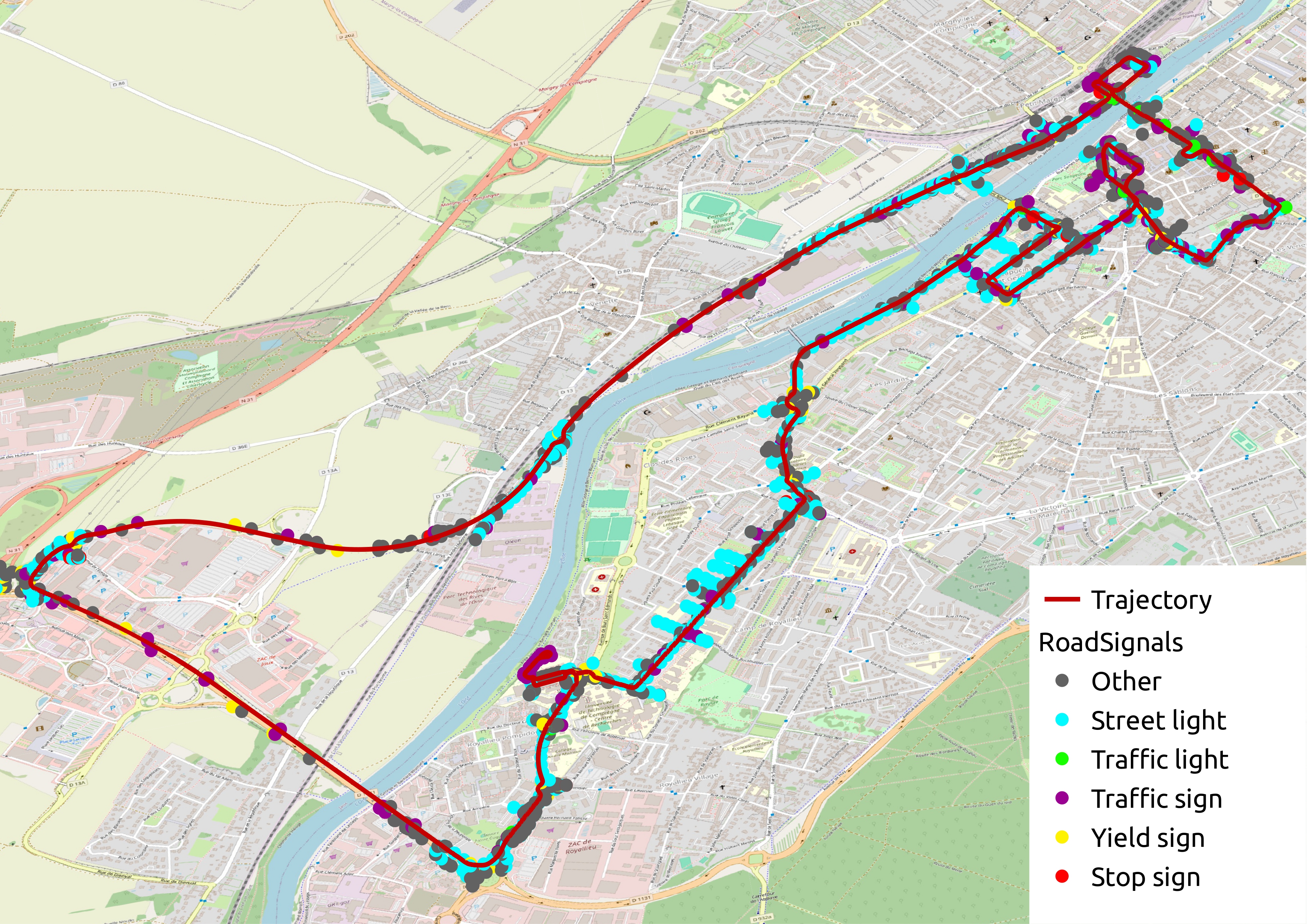
Compiegne HD Map
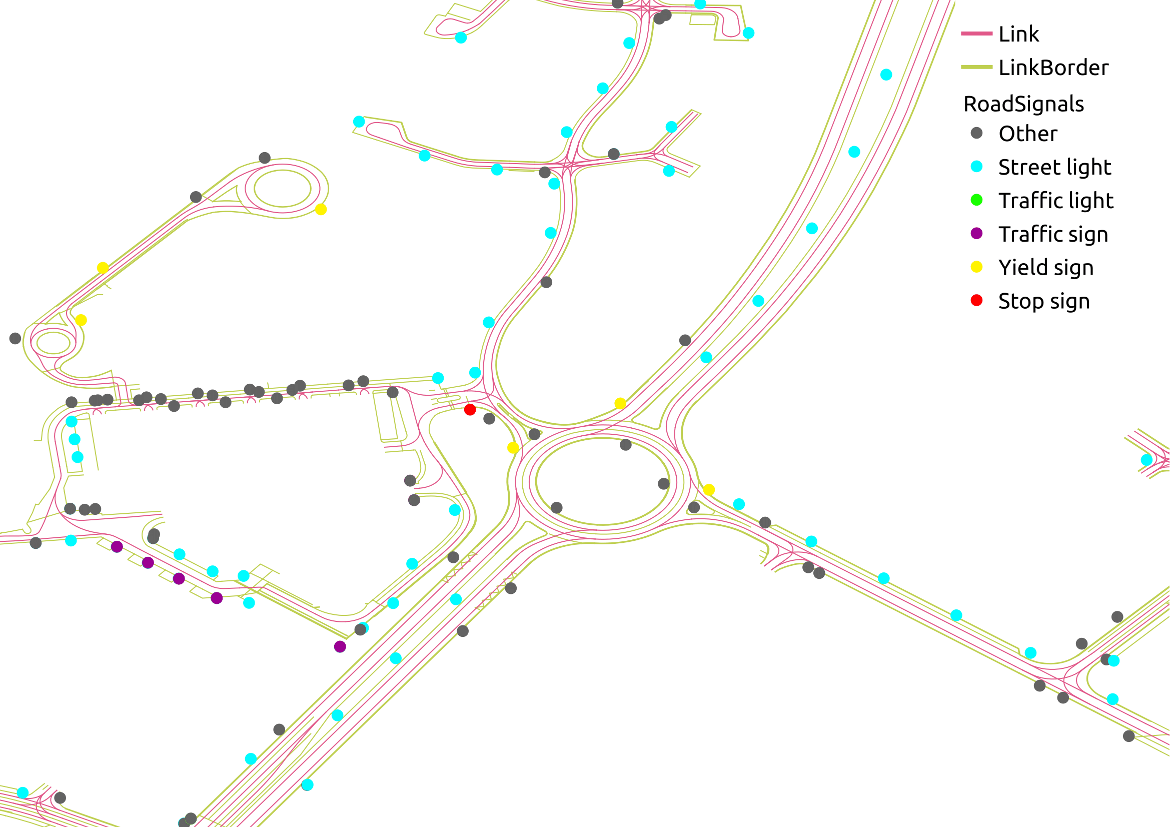
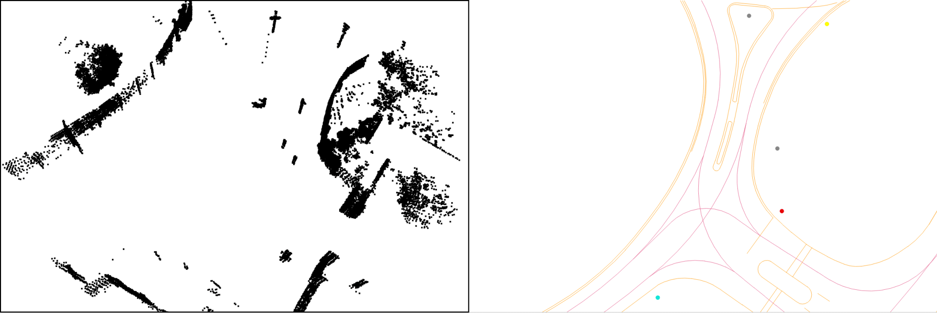
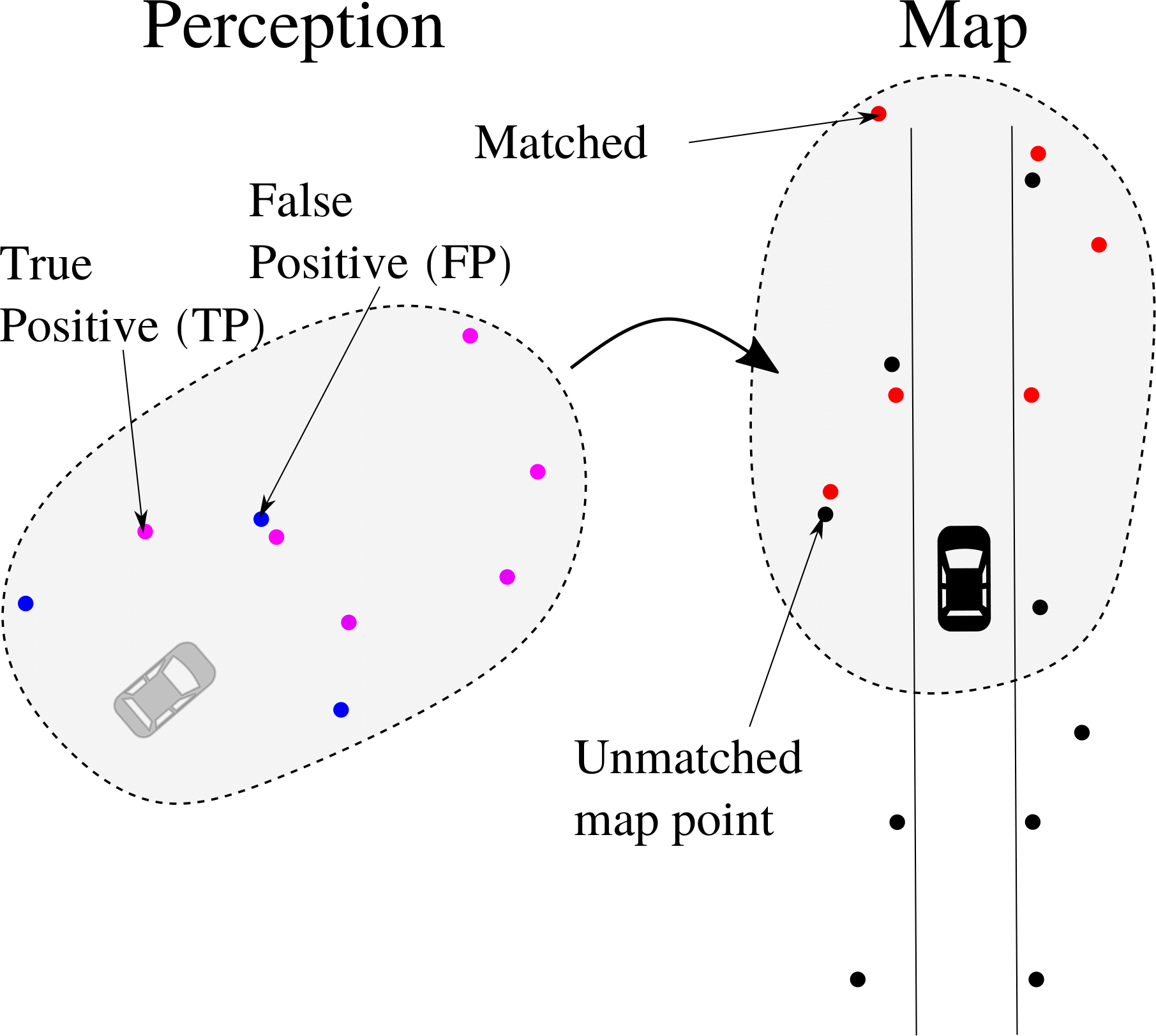
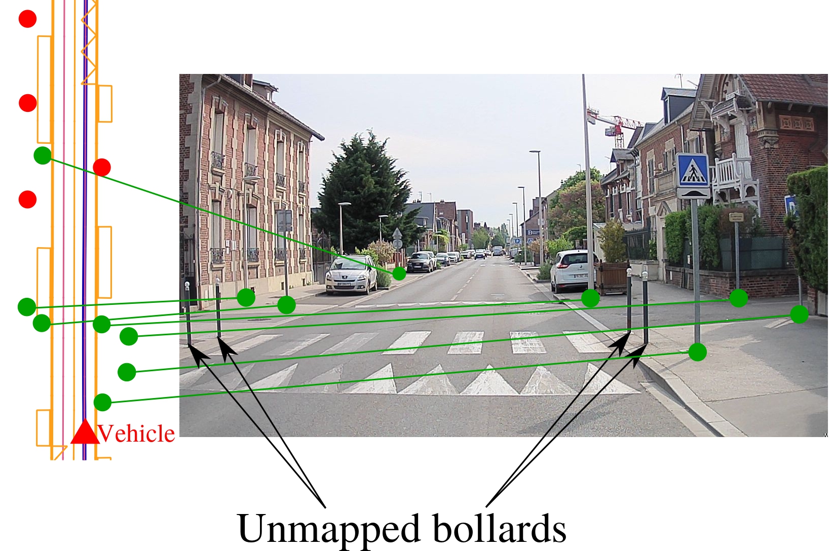
Localization with vector maps
Indiscernible features ⇒ Data association
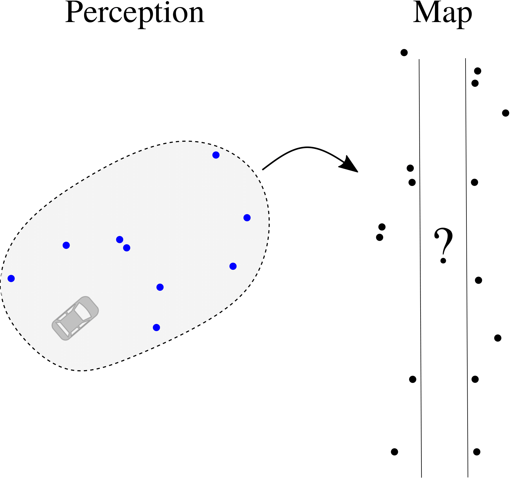
Indiscernible features ⇒ Data association
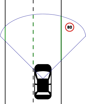
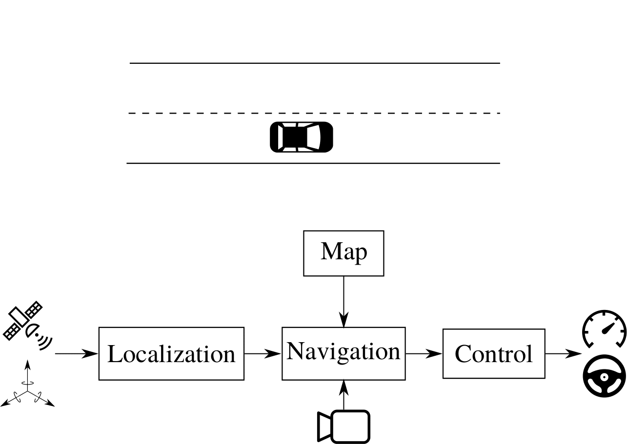
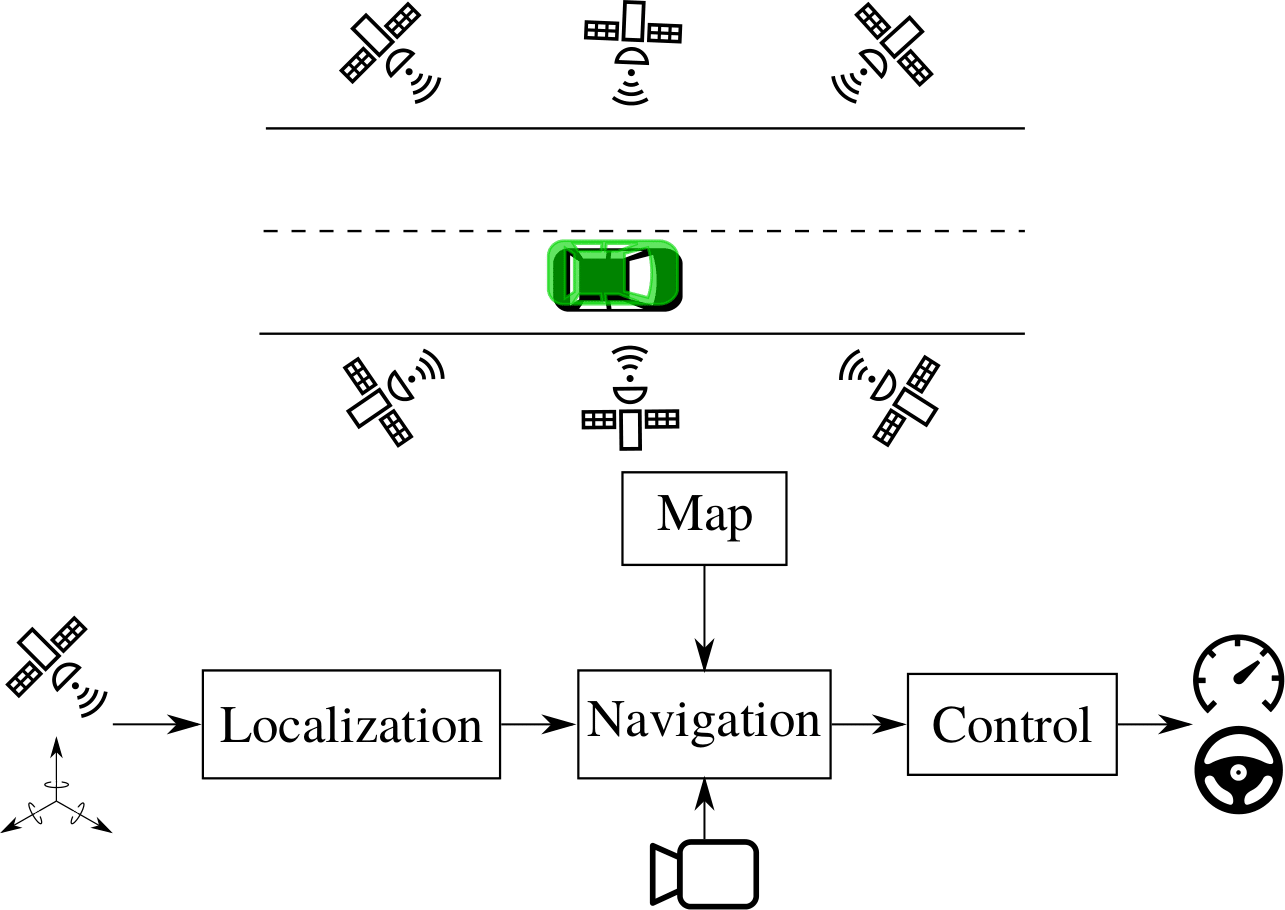
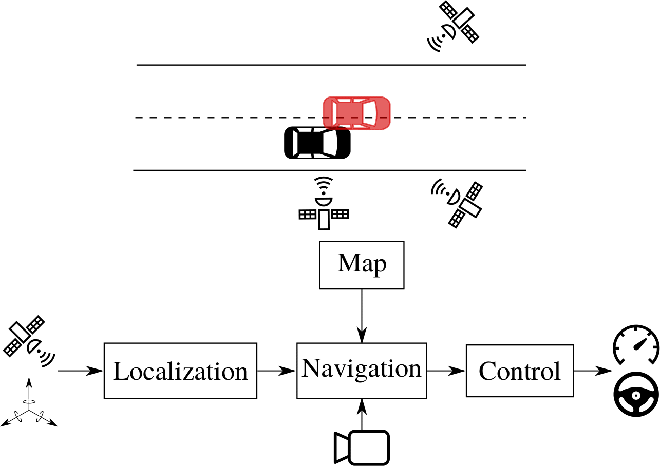
Studied AD pipeline
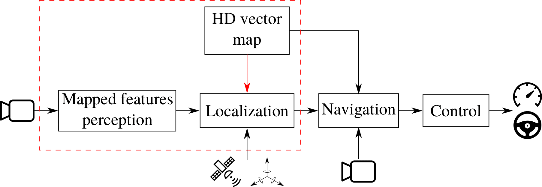
Mapped features detection
Geometric approaches
- 👍 Limited data needed
- 👎 Expert tuning
- 👎 Missdetections, false positives (trunks, corners, …)
Machine learning
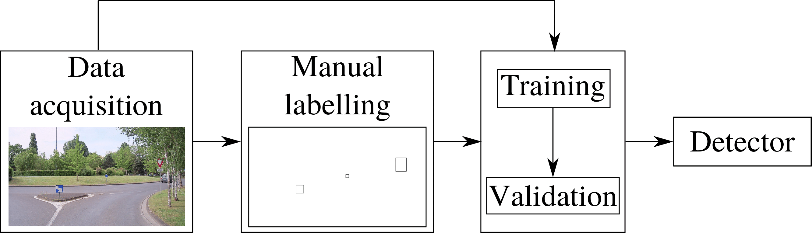
- 👍 Better performance
- 👍 Less tuning, better genericity
- 👎 Huge amount of data needed
- 👎 Labelling
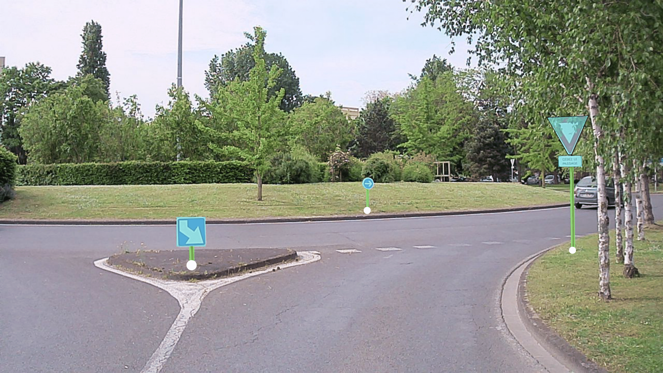
Case study: poles for localization
- Map for localization
- Maximize map usage -> poles common in road environments
- Minimize risks of false detections -> map-specific detection
- Machine learning for detection
- Minimize or avoid human labelling
- Leverage maps for automatic annotation
- Multi-sensor post-processing for automatic annotation
- Training with automatic annotations
- Uncertainty handling
- Minimize or avoid human labelling
- Localization using trained detectors without human input
Map-aided annotation
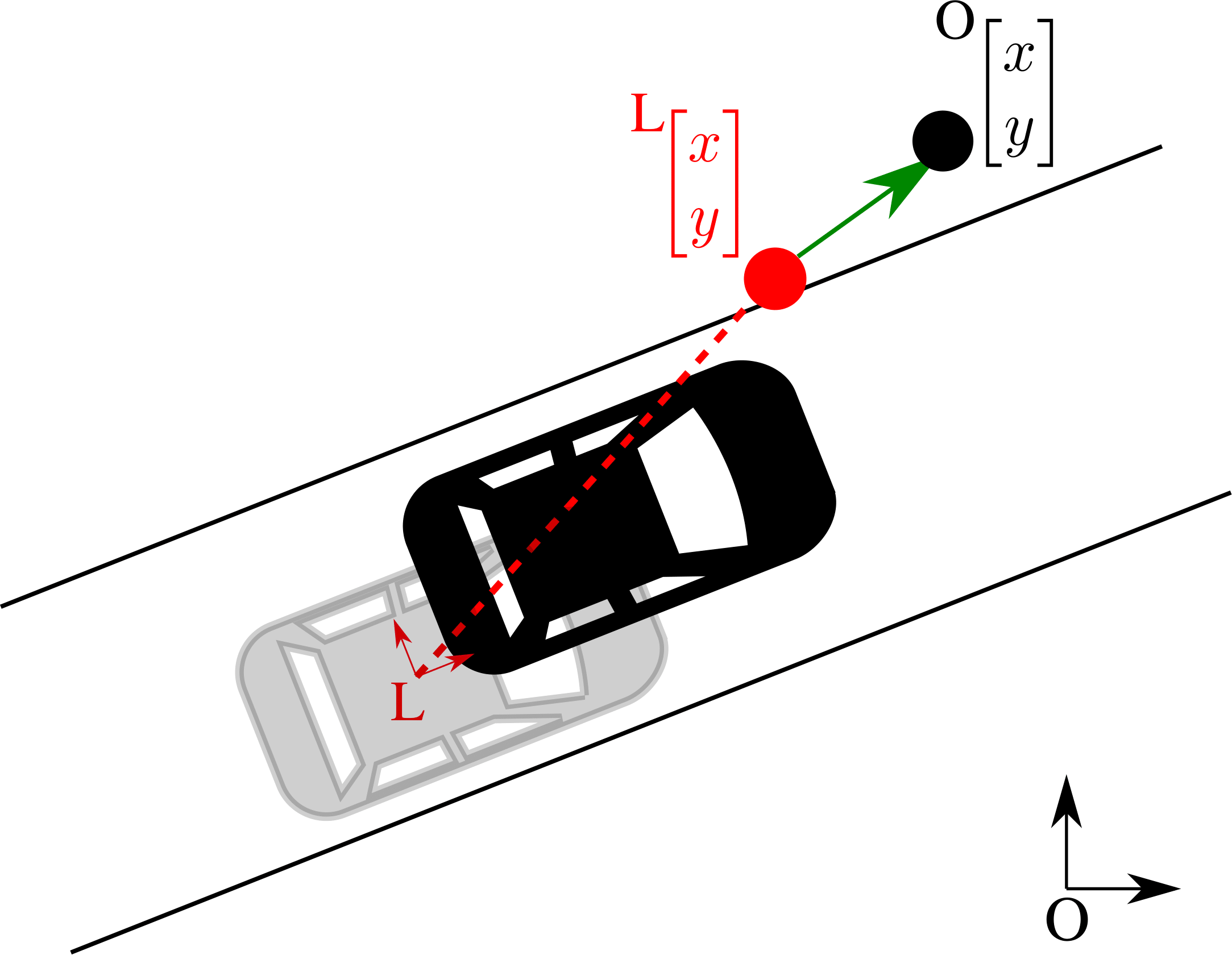
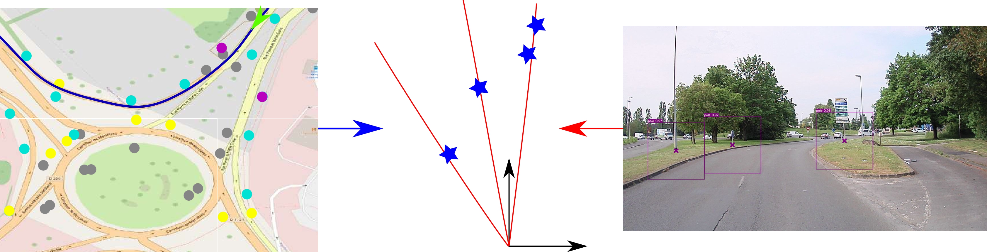
2D map projection with localization reference
 Naive projection
 Projection error source
Lidar refinement
 Ground estimation and annotation projection
 Occluded pole bases removal
Dataset and evaluation metrics
- Multiple sequences around Compiegne
- 2,830 images manually annotated
- 9,017 poles
Multi-modal annotation
Lidar-based annotation
 Initial image
 Corresponding point cloud
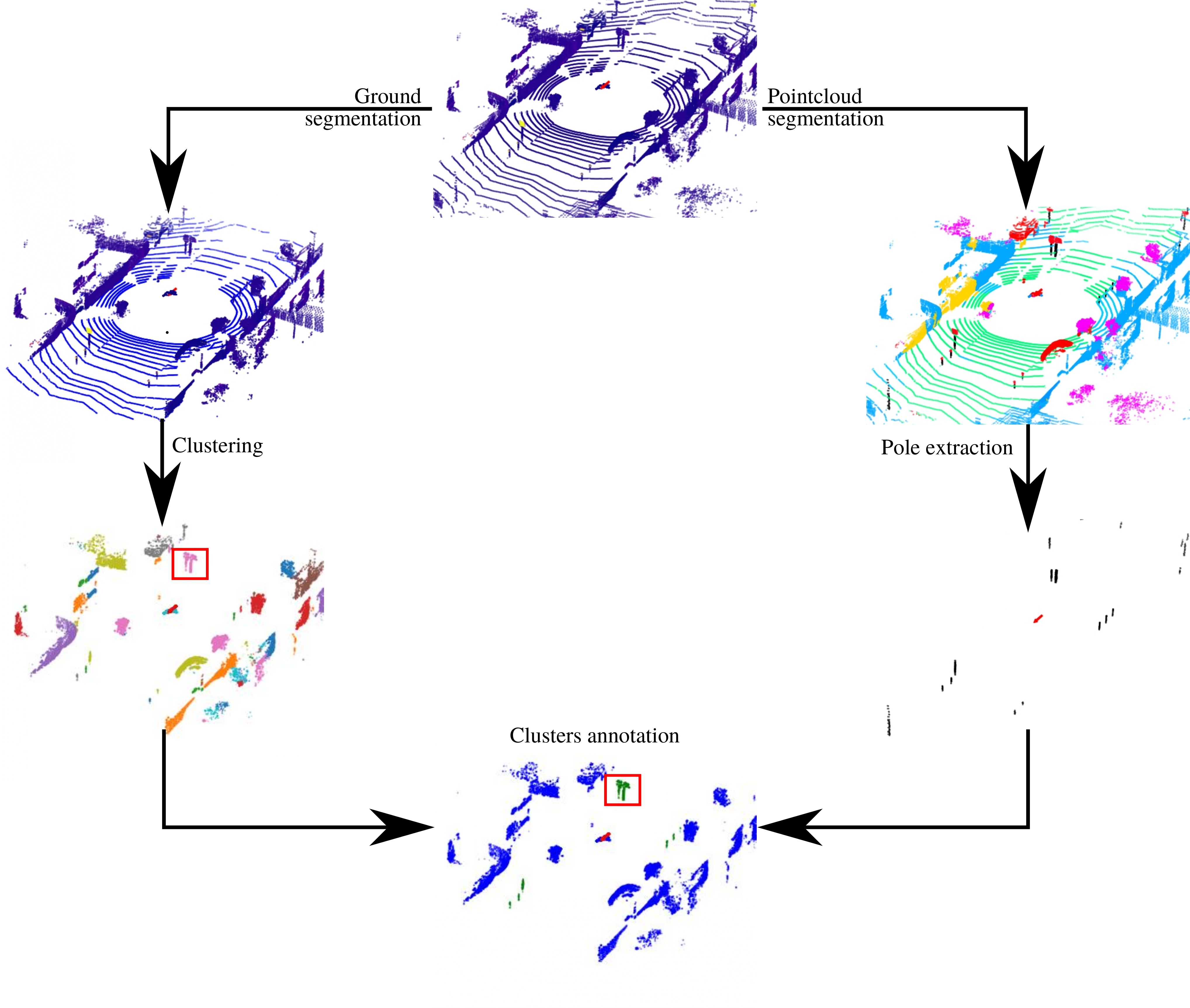
Lidar-based annotation
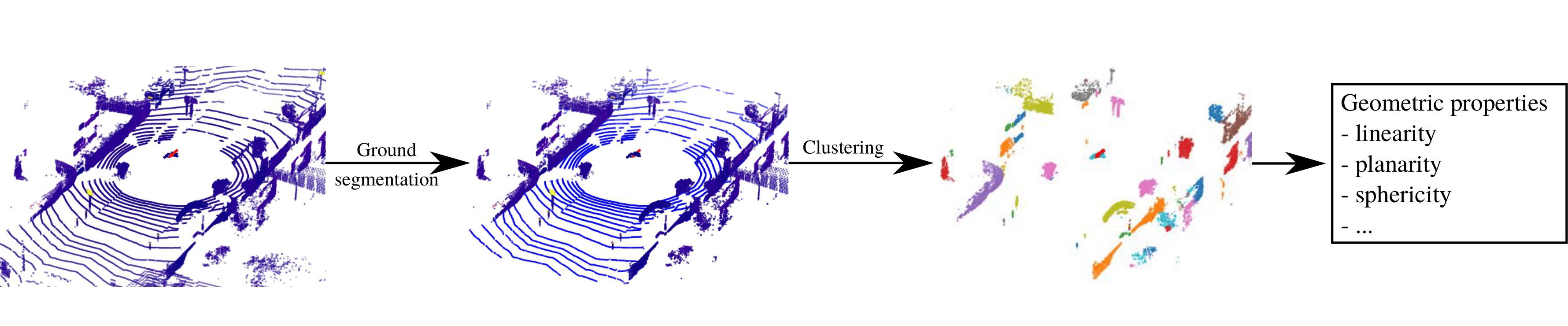
 Pointcloud segmentation
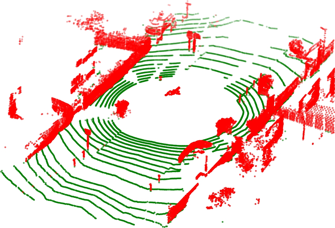 Ground segmentation (more precise)
X. Zhu et al., “Cylindrical and asymmetrical 3d convolution networks for lidar segmentation”. In Proceedings of the IEEE/CVF conference on computer vision and pattern recognition. 2021.
Segmentation-based annotation
Initial image
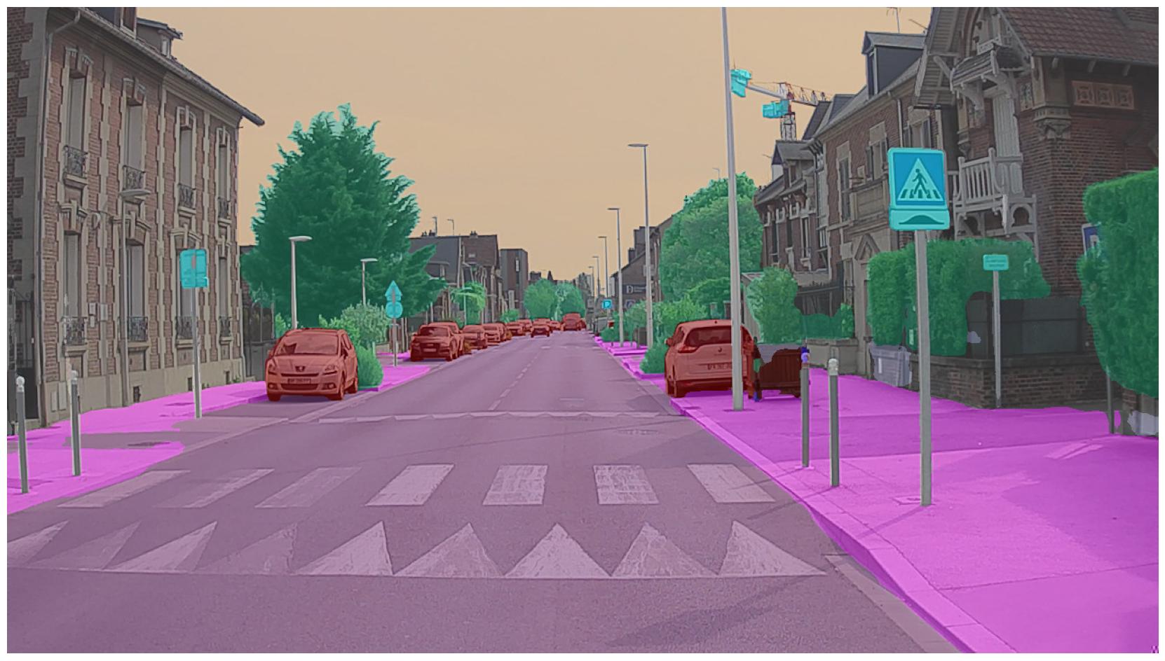 Segmentation mask
J. Wang et al., “Deep High-Resolution Representation Learning for Visual Recognition,” In IEEE Transactions on Pattern Analysis and Machine Intelligence, vol. 43, no. 10, pp. 3349-3364, 1 Oct. 2021.
Segmentation-based annotation
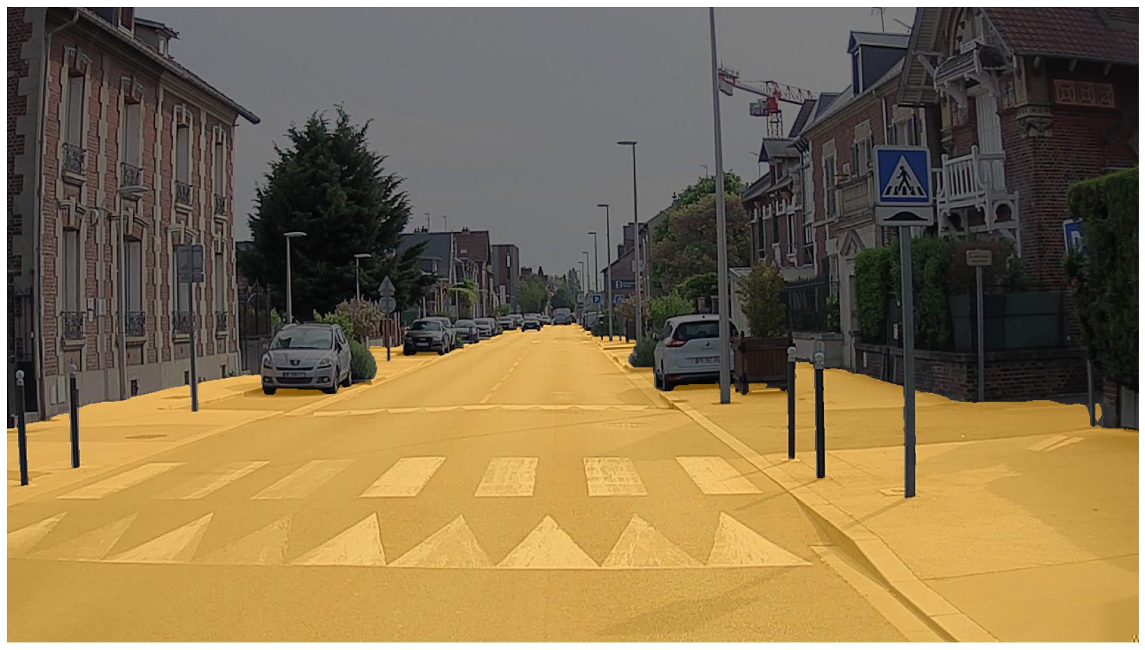 Ground mask
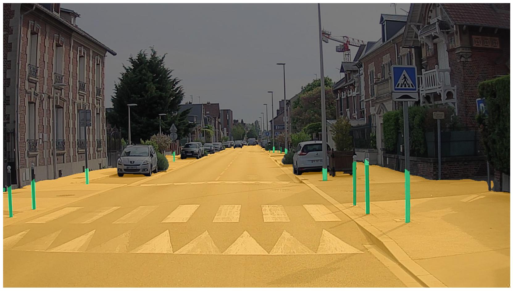 Ground + pole bases mask
J. Wang et al., “Deep High-Resolution Representation Learning for Visual Recognition,” In IEEE Transactions on Pattern Analysis and Machine Intelligence, vol. 43, no. 10, pp. 3349-3364, 1 Oct. 2021.
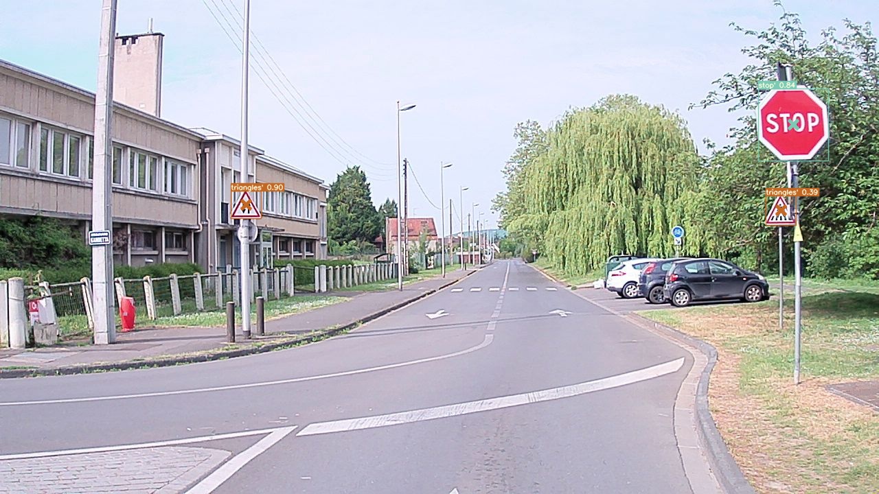
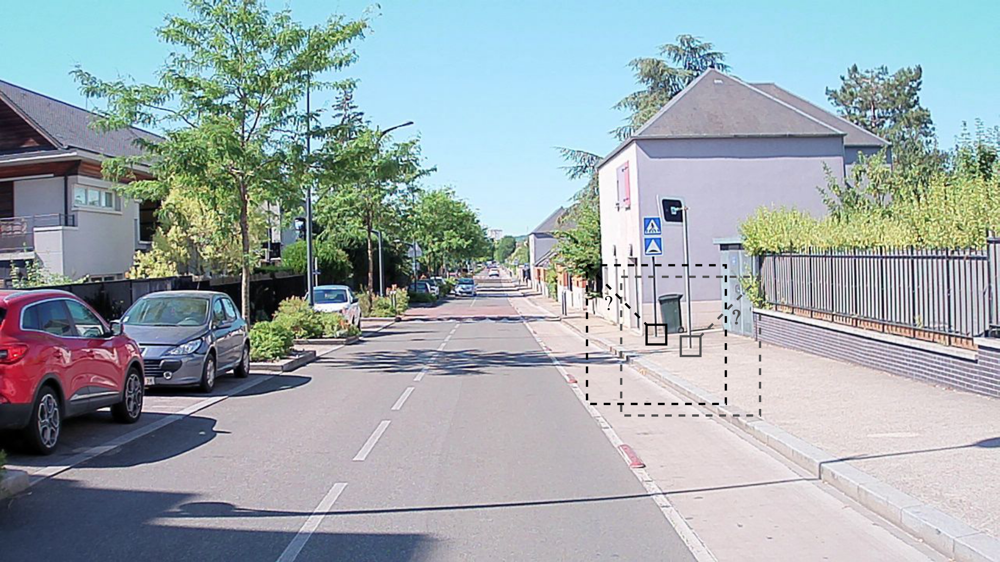
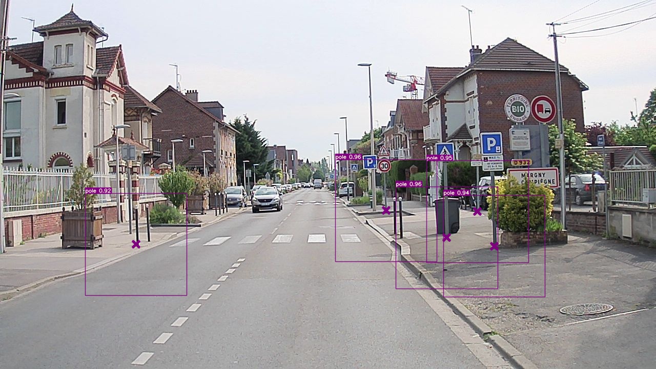
Pole base detection for cameras
- Pole base detection using object detection
- Based on YOLOv7 network
- Bounding box = visual context
- Automatic annotation: Prone to errors (missed objects, false positives)
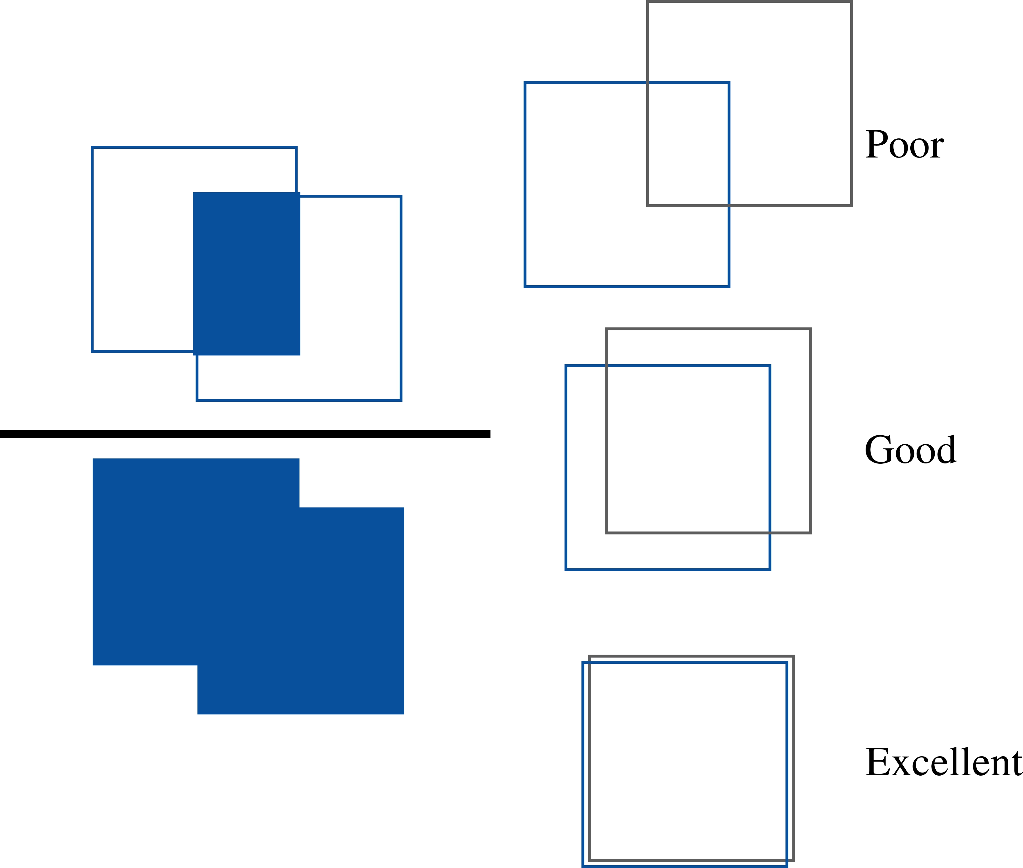
Evaluation metrics
- Precision, Recall
- Intersection-over-Union (IoU)
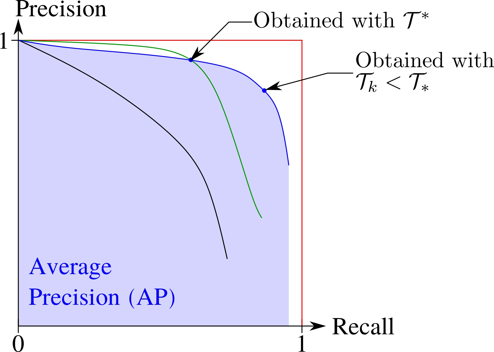
- Average Precision
- Mean horizontal Absolute positioning Error: MAE-x
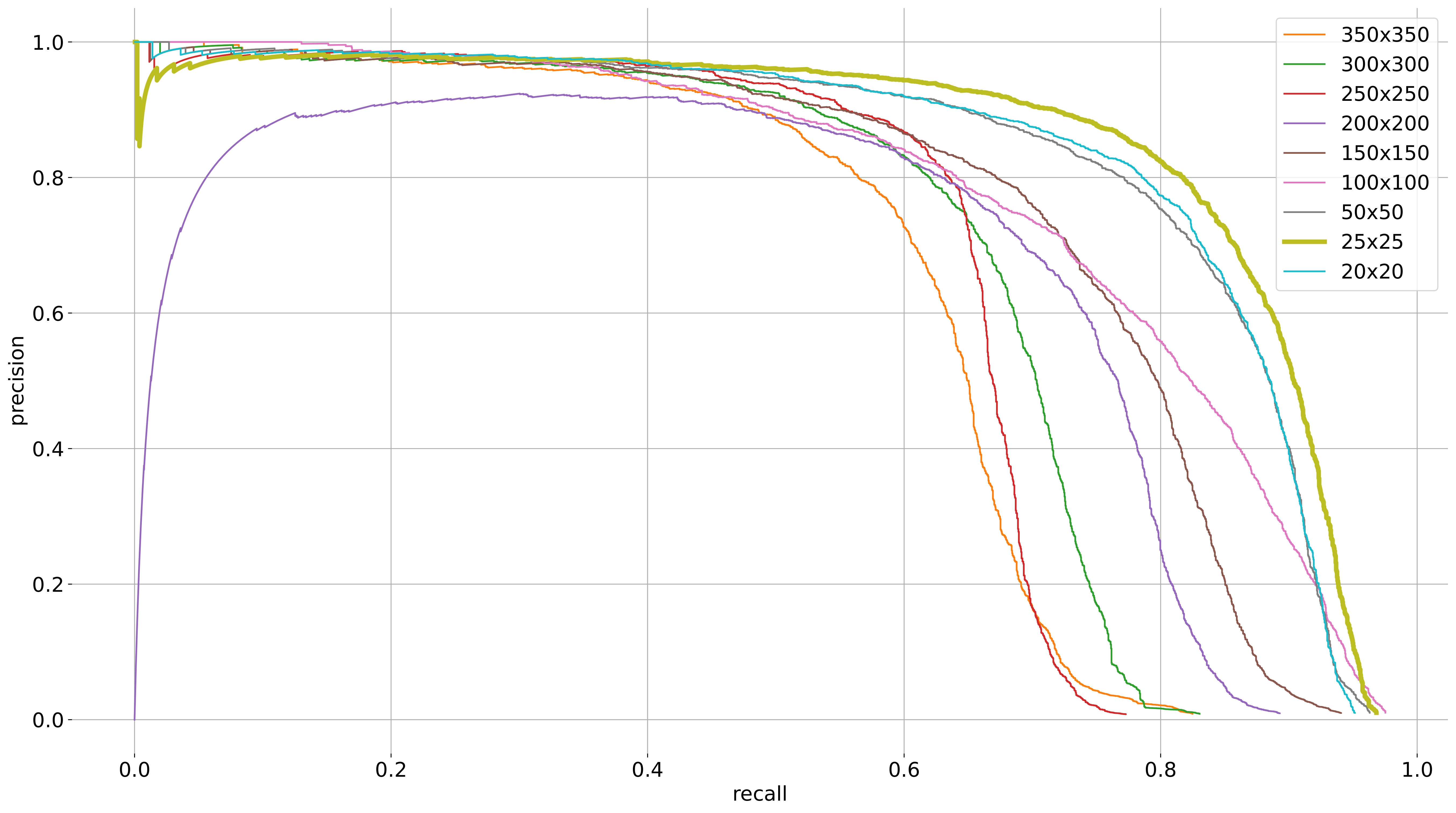
Precision-Recall curve
Map-based pole base detection learning
- Training set: 5391 images
- Validation set: 2830 images manually annotated
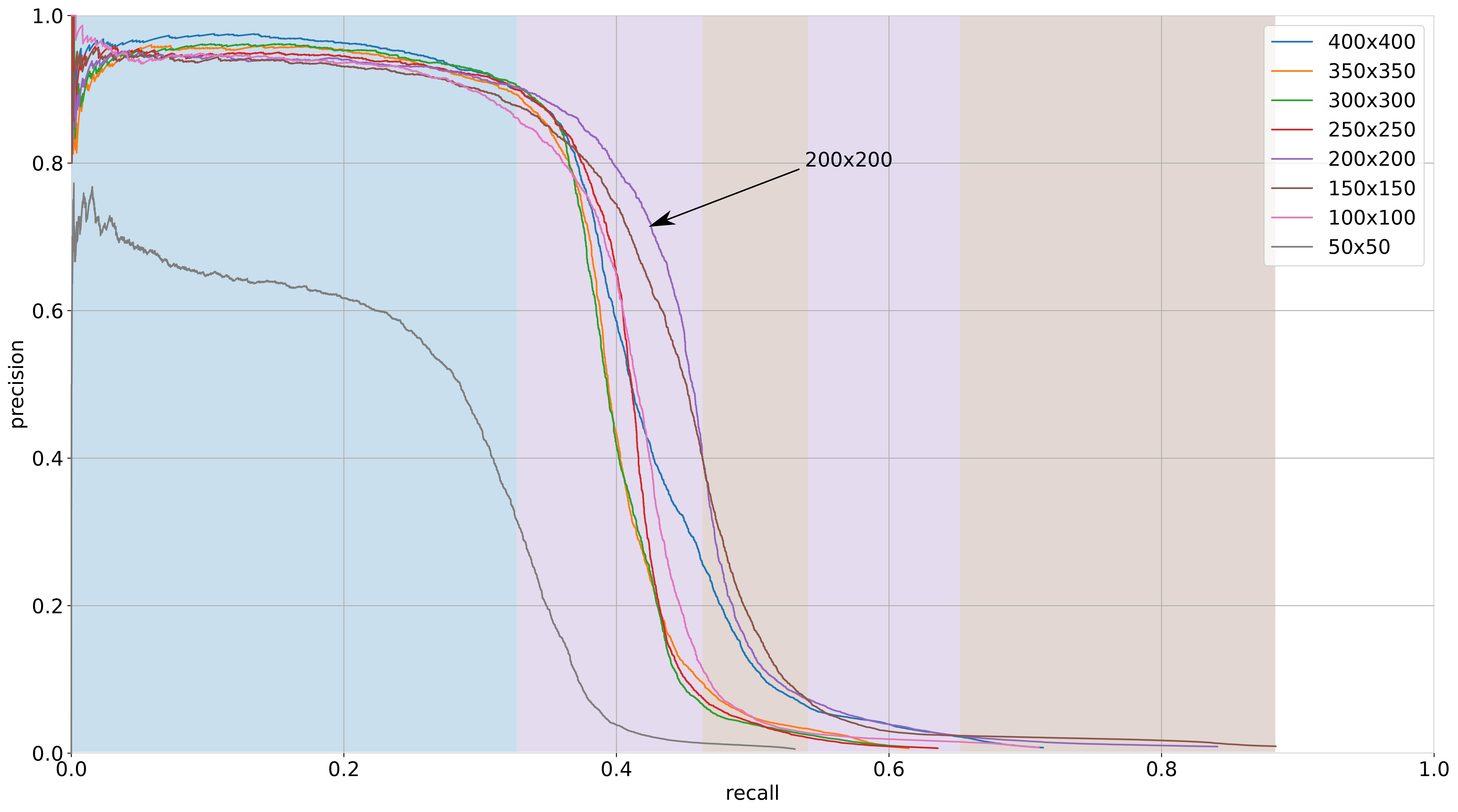
| Box | 50x50 | 100x100 | 150x150 | 200x200 | 250x250 | 300x300 | 350x350 | 400x400 |
|---|---|---|---|---|---|---|---|---|
| AP % | 21.2 | 39.2 | 42.5 | 43.2 | 38.9 | 38.3 | 38.4 | 41.3 |
| MAE-x (px) | 4.01 | 5.84 | 8.90 | 10.84 | 11.76 | 14.97 | 18.2 | 24.30 |
Multi-modal automatic annotation method for learning
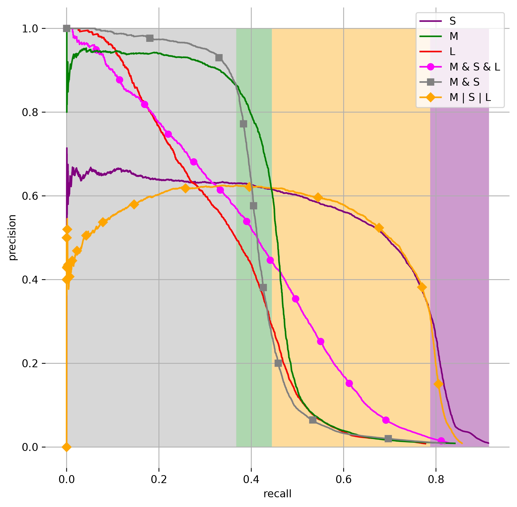
Uncertainty management
- Annotations used for training: Intersection of annotation sets
- Ambiguous cases: Union of annotation sets
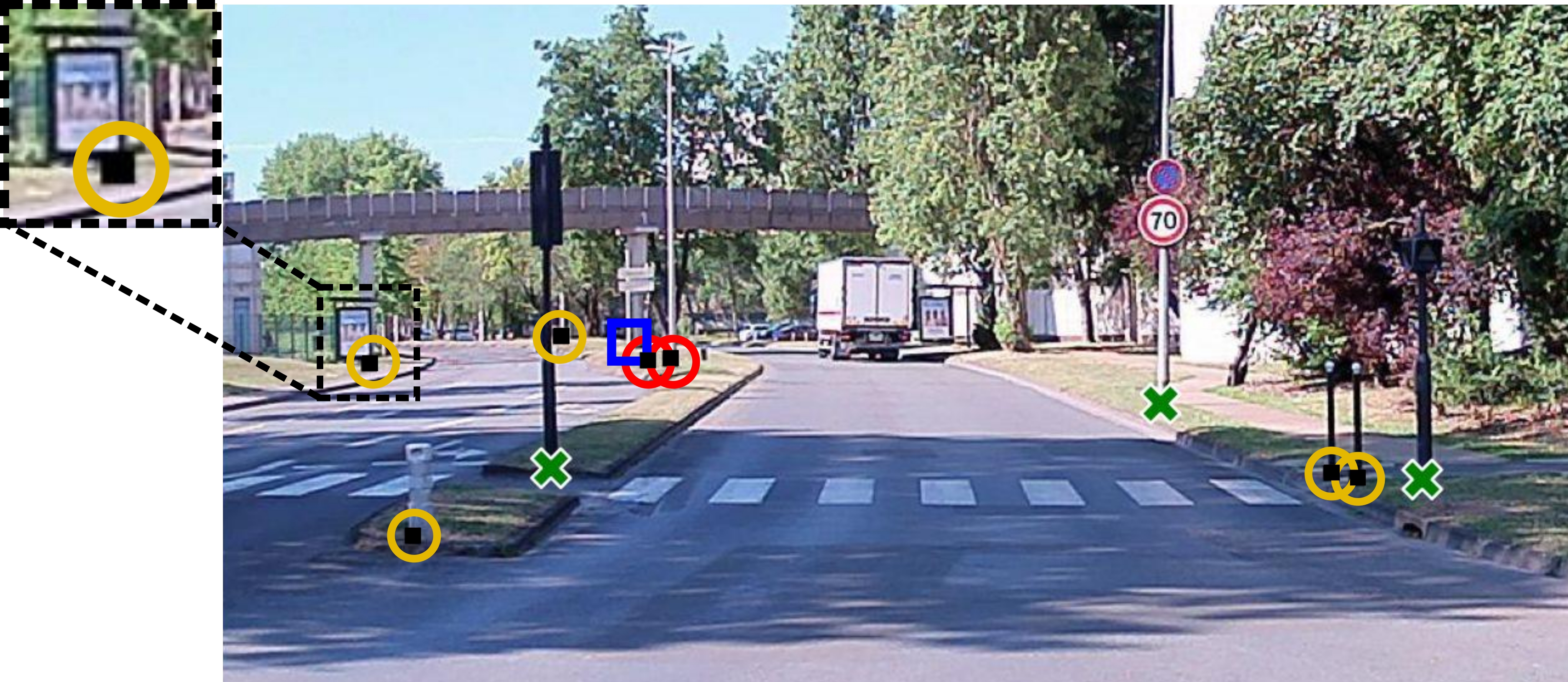
Learning with uncertainty management
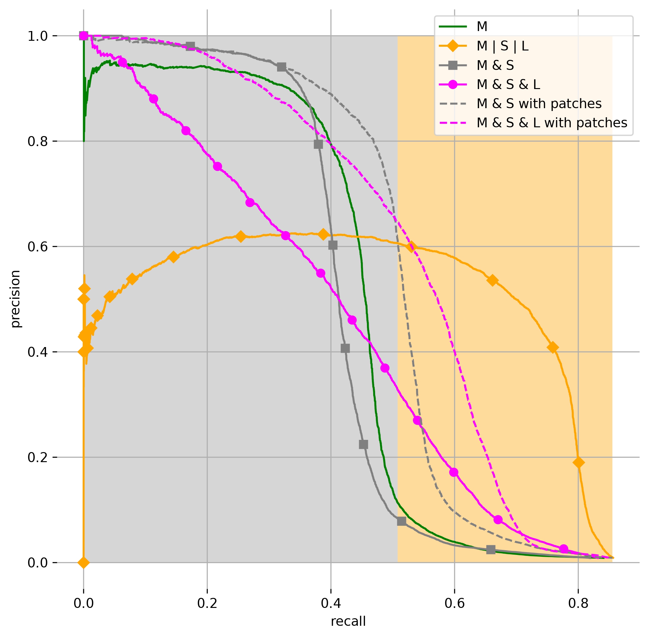
Available detectors
.jpg)
.jpg)
.jpg)
- Integration to a GNSS + Dead Reckoning sensors system
- Combinations: F and All
| Model | M95 | MS95 | M90 | MS90 |
|---|---|---|---|---|
| Precision (%) | 95 | 95 | 90 | 90 |
| Recall (%) | 4.3 | 30.4 | 33.3 | 38.5 |
Pole-based localization
- Camera observations
- Lack of depth → map features projected into camera frame
- Use angles for observations and map features in camera frame
- Pose and calibration errors impact
Data association
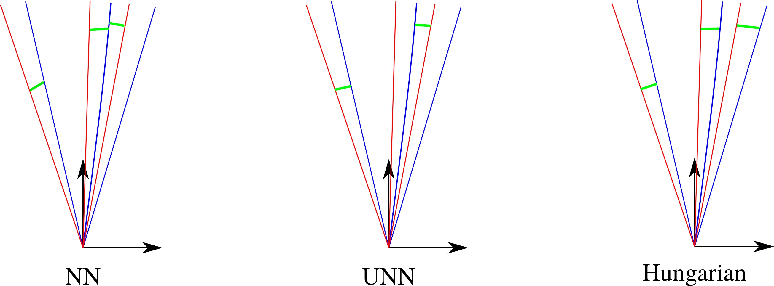
- Avoid wrong associations: gating
- Hungarian chosen
Nominal scenario
- Extended Kalman Filter
- Dead reckoning: 4-wheel speed + yaw rate model
- GNSS: SPP pose estimation
- Tightly-coupled cameras
- 50Hz pose estimation frequency
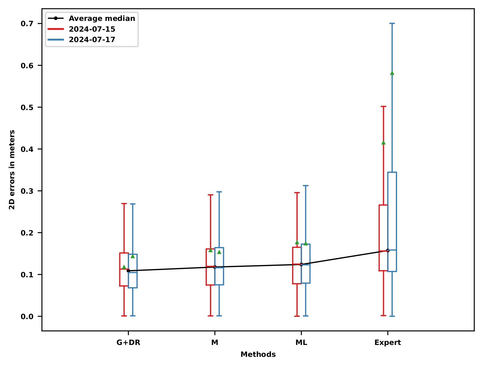
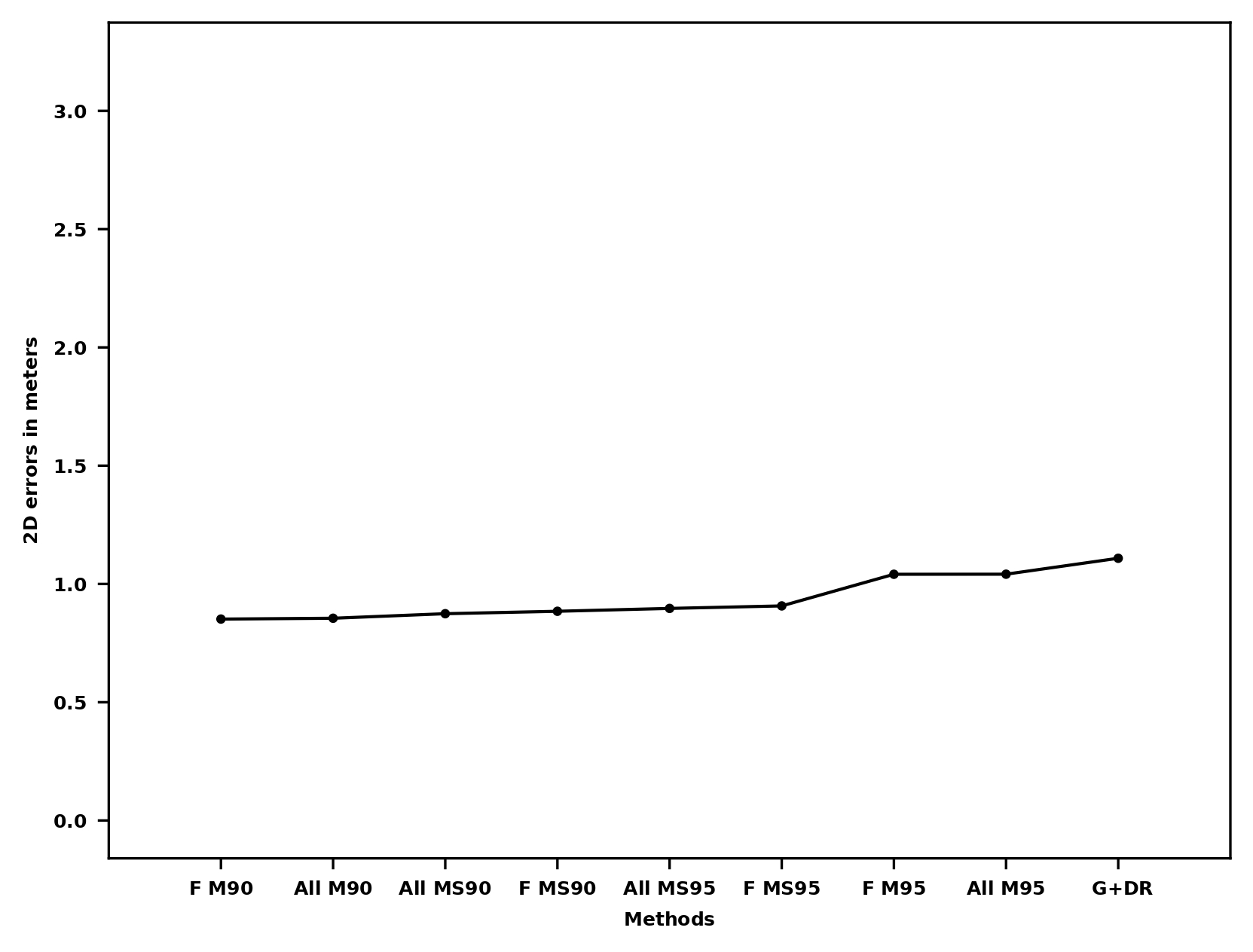
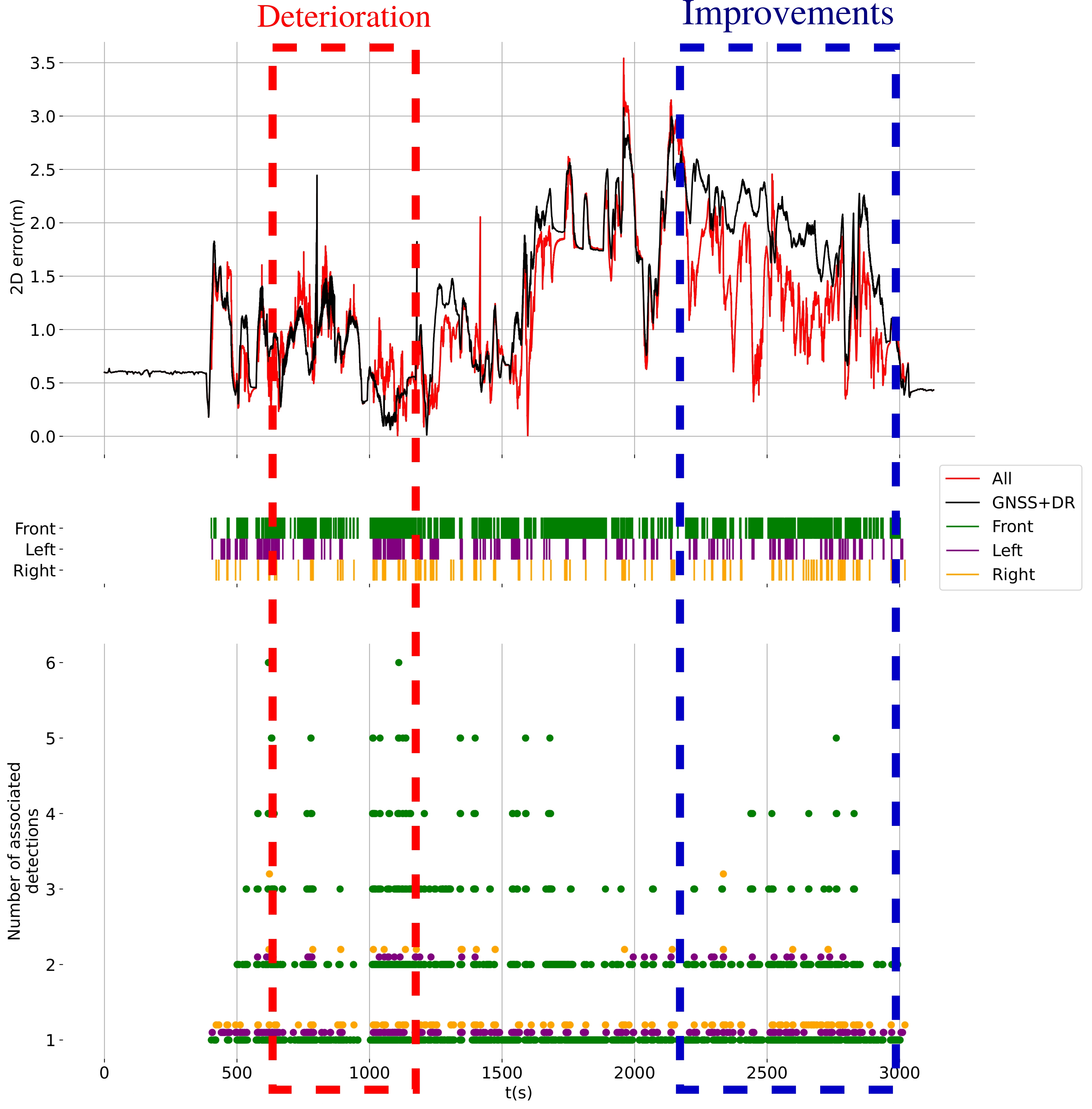
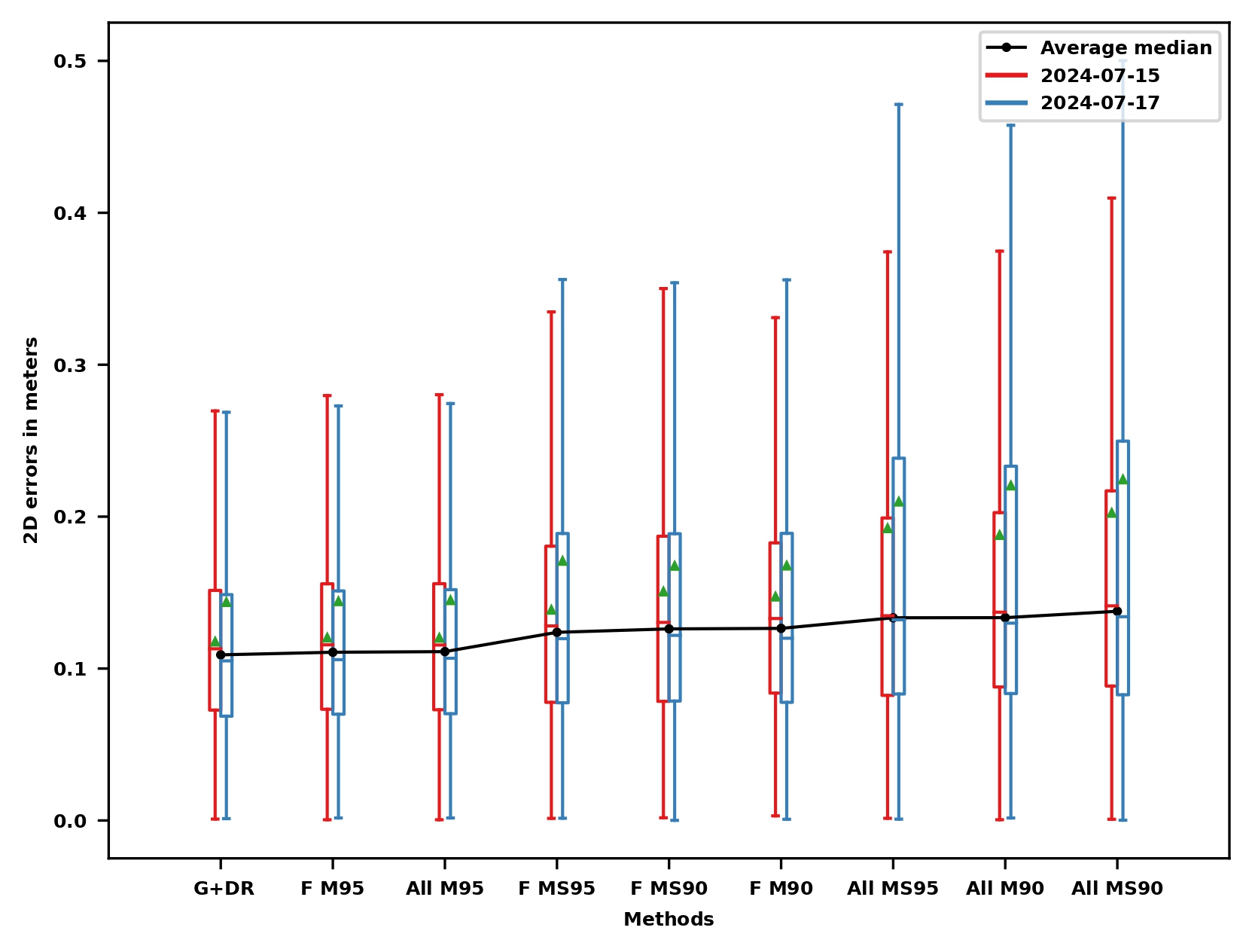
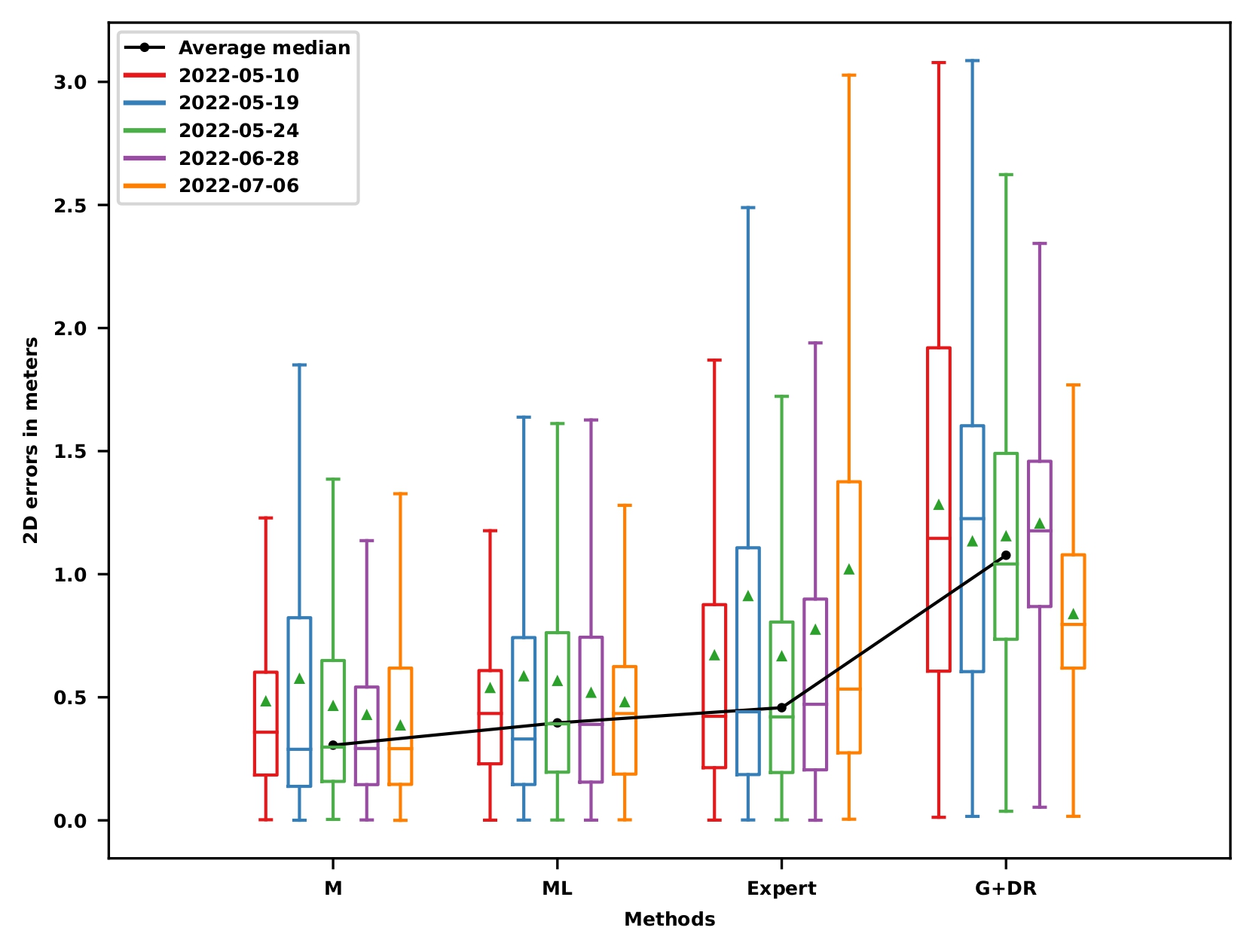
Localization results

Localization results
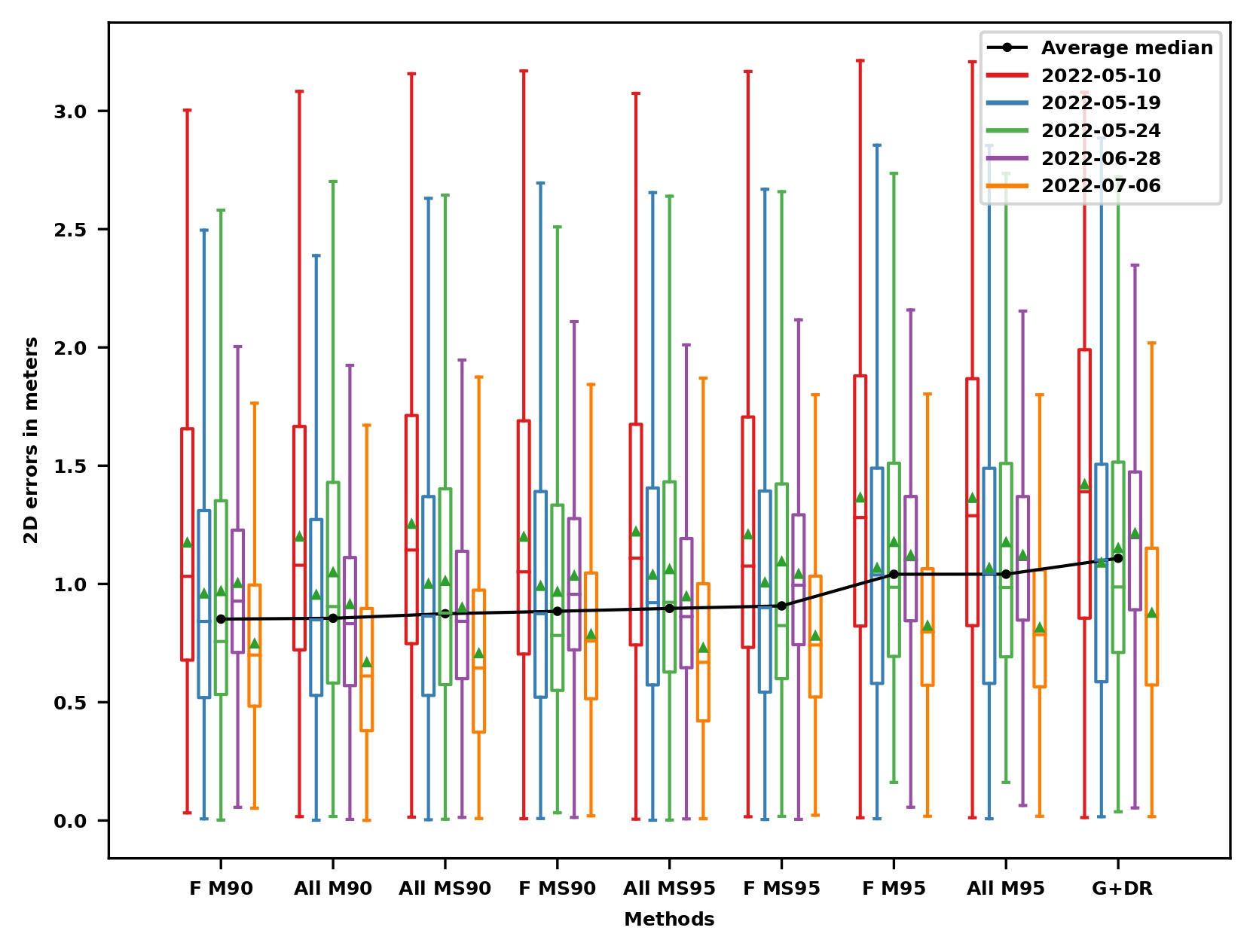
Localization results
Performance limitations
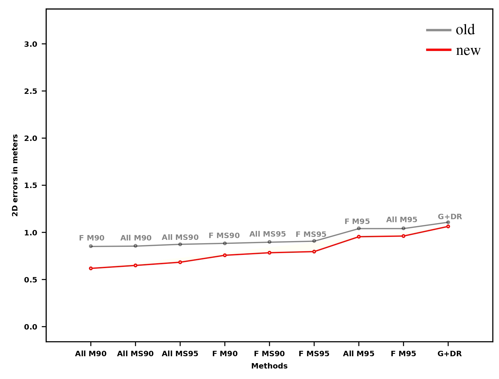
Better prior pose for data association improvements
Learning on manually annotated data
- Higher recall reachable
- Optimal box size: 25x25
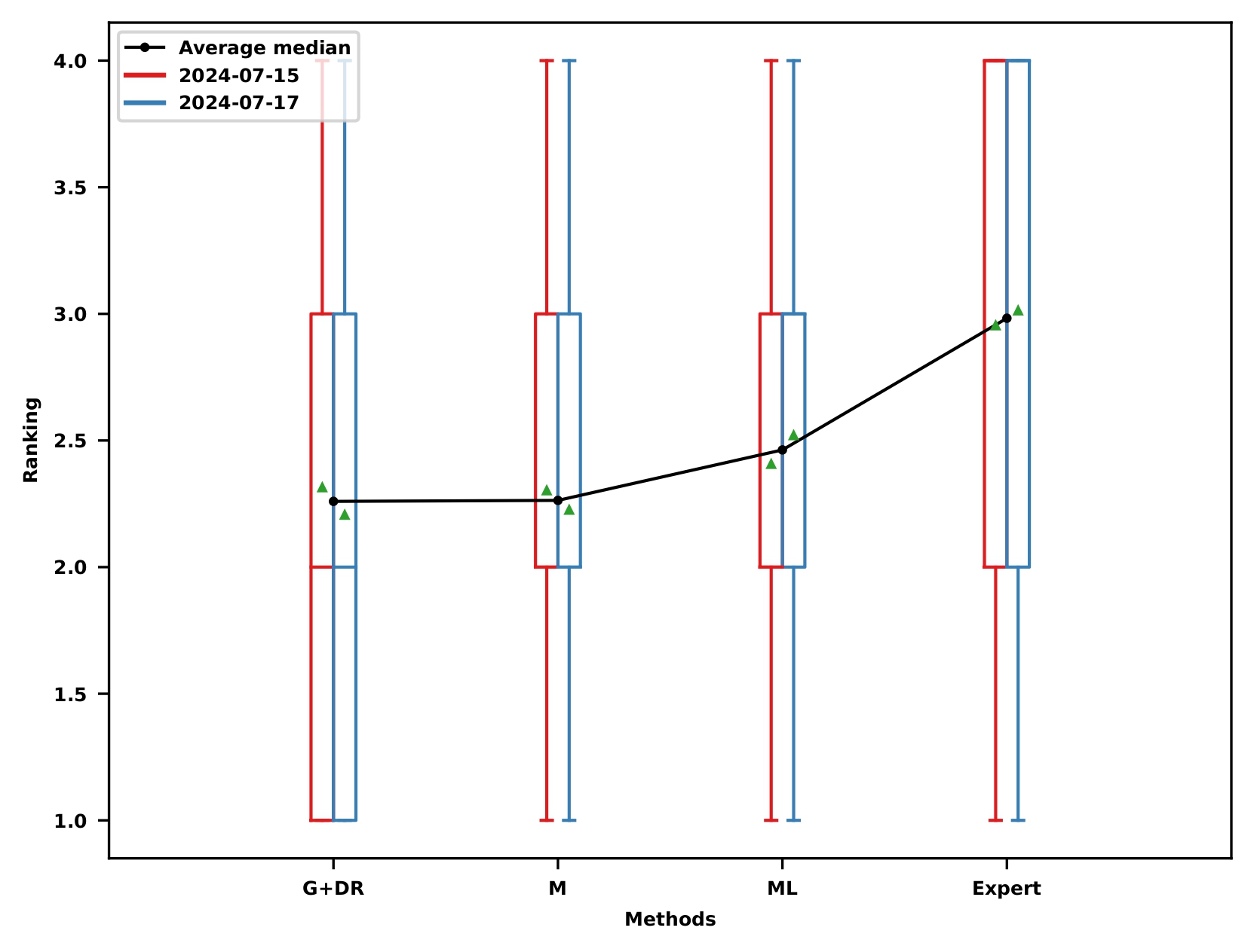
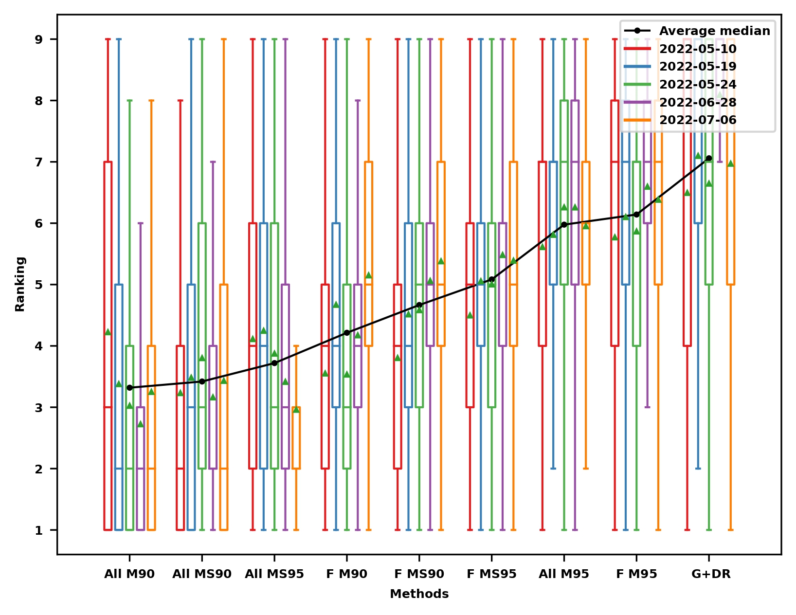
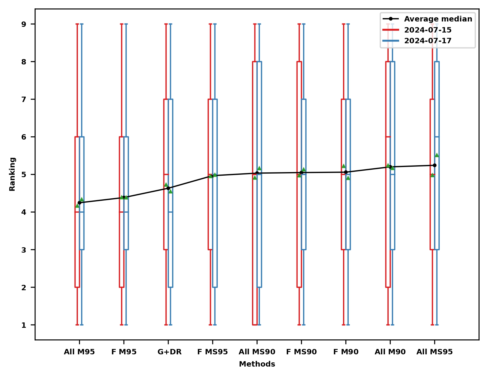
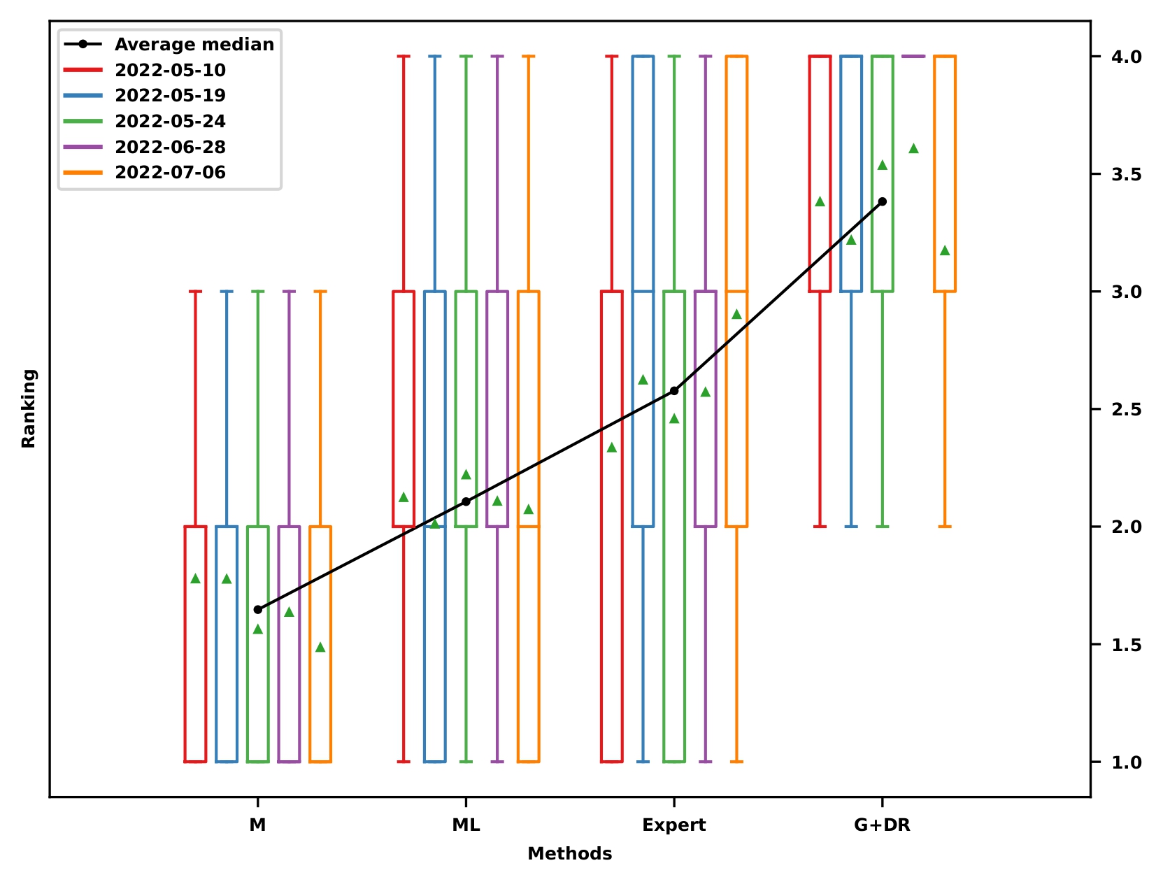
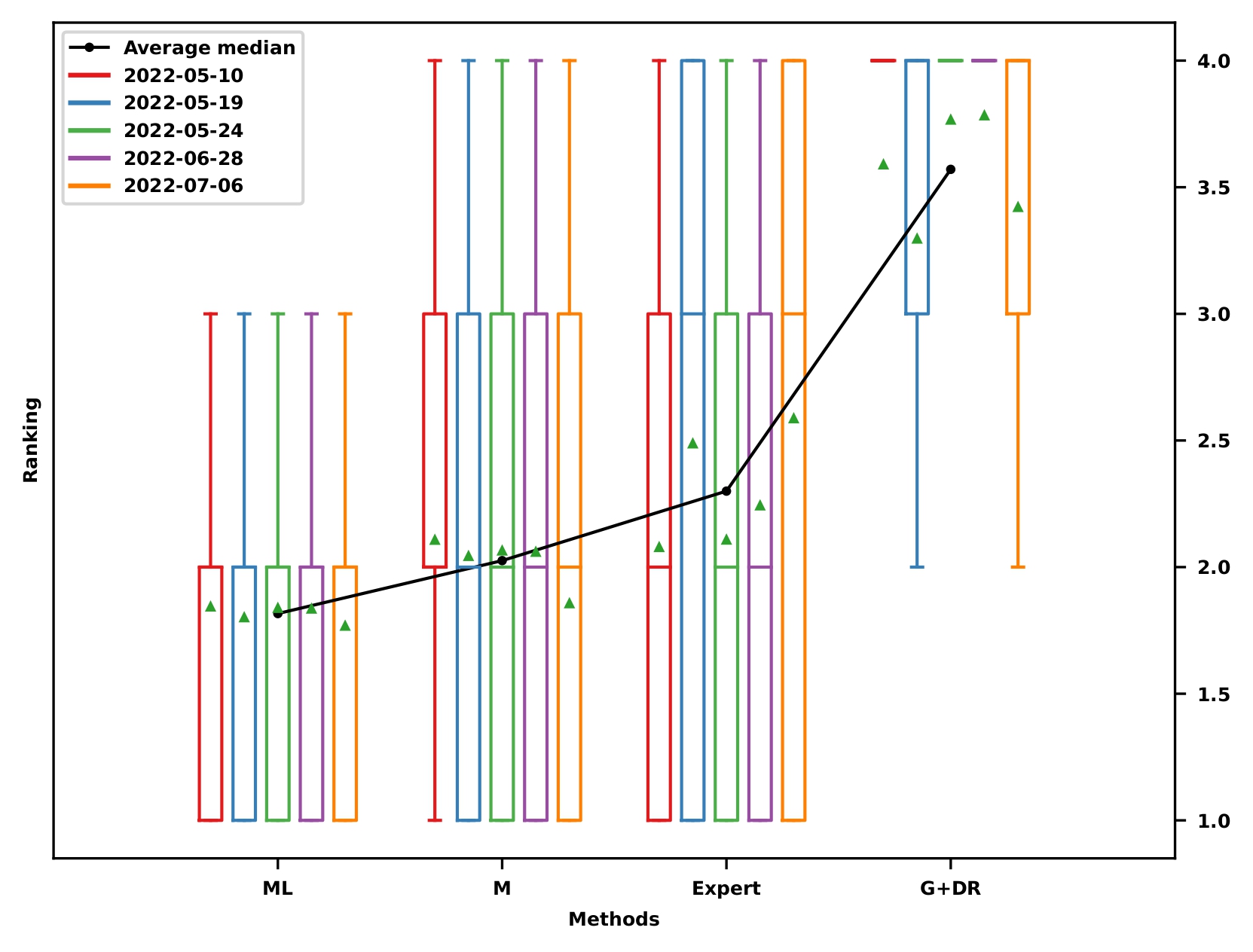
Localization results: Ranking
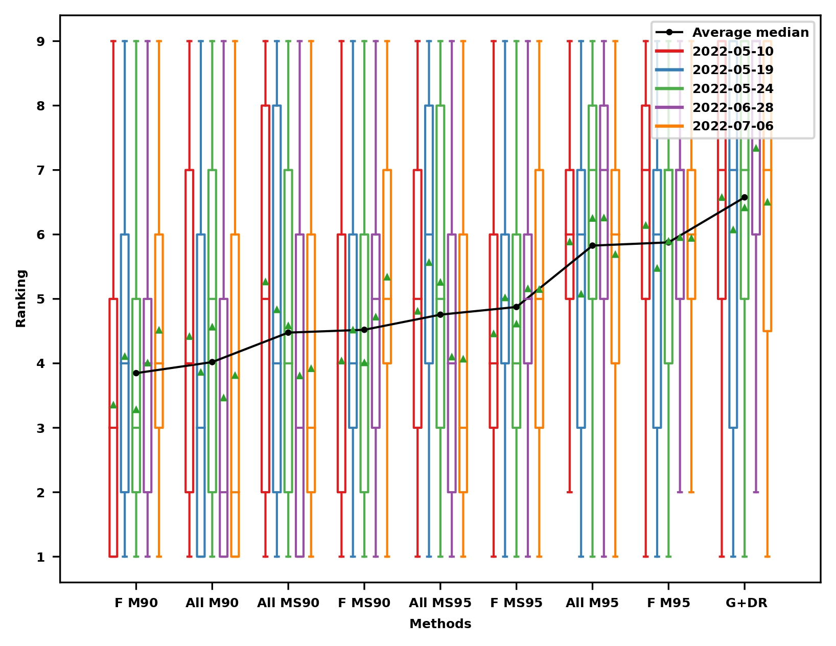
Localization reference for data association: Ranking
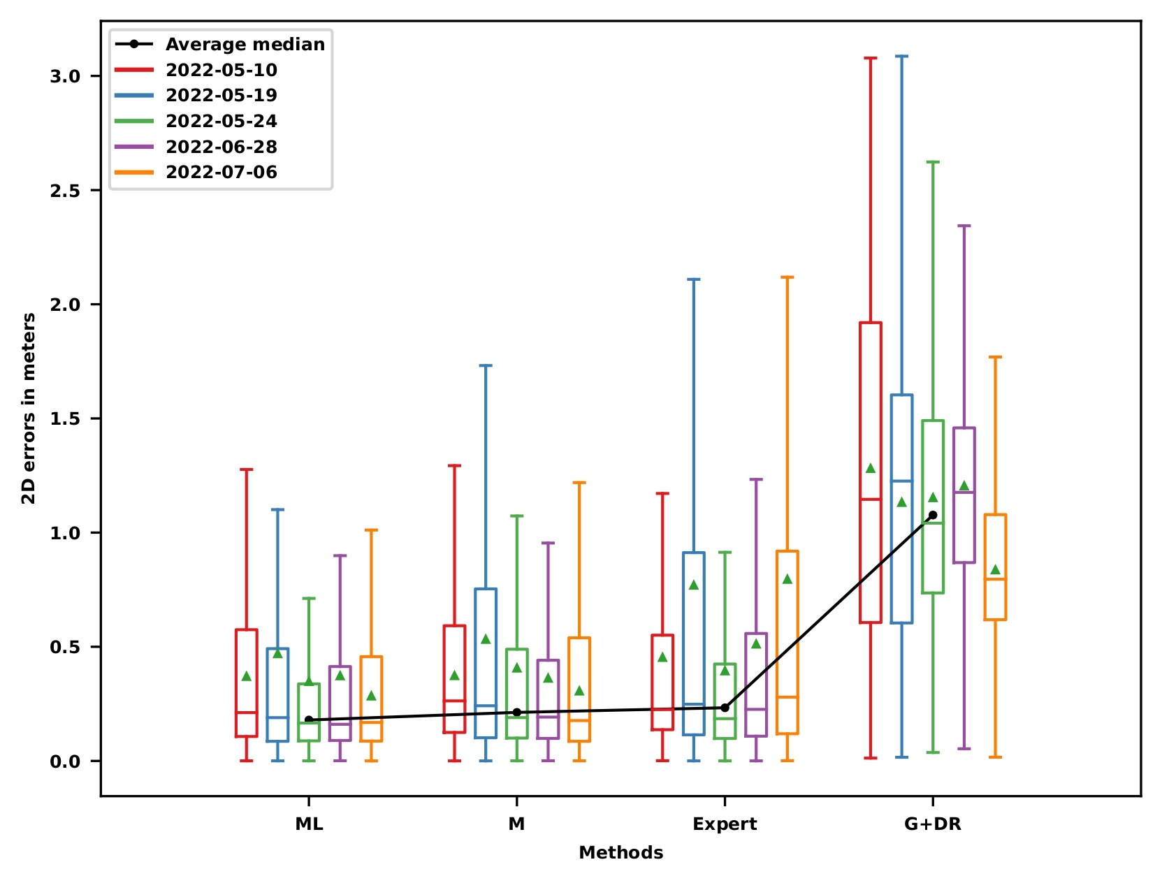
Results with PPP-RTK
Lidar: Map-based annotation
- Data association between map points and clusters
Lidar: Lidar-based annotation
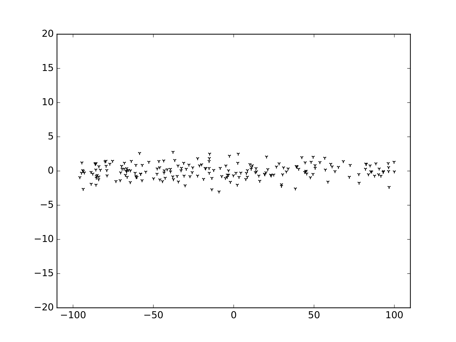
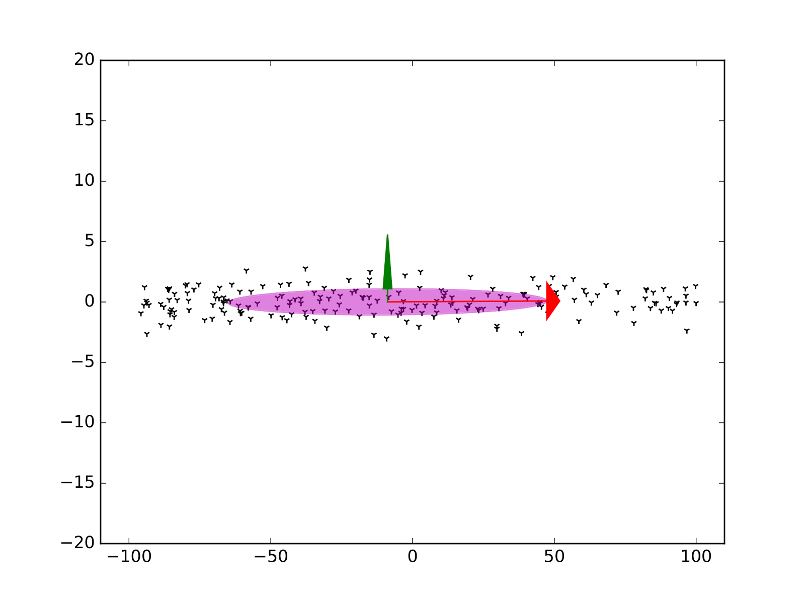
Lidar: Principal Component Analysis (PCA)
Points \[ X = \begin{pmatrix} x_0 & x_1 & \dots & x_N \\ y_0 & y_1 & \dots & y_N \end{pmatrix} \]
Mean
\[ \bar{X} = \begin{pmatrix} \bar{x} \\ \bar{y} \end{pmatrix} \]
Lidar: PCA - Covariance matrix
\[ Cov = \frac{ \left(X - \bar{X}\right) \cdot \left( X - \bar{X} \right)^T }{ N - 1 } \]
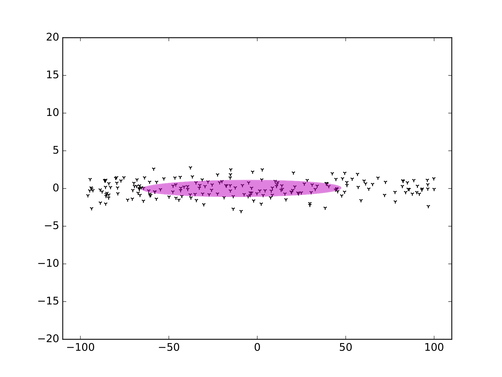
Lidar: PCA - Eigenvectors and eigenvalues
\[ Cov = Q \cdot \Gamma \cdot Q^{-1} \]
\[ Q = \begin{pmatrix} \color{red}{v_1^x} & \color{green}{v_2^x} \\ \color{red}{v_1^y} & \color{green}{v_2^y} \end{pmatrix} \]
\[ \Gamma = \begin{pmatrix} \color{red}{\sigma_1^2} & 0 \\ 0 & \color{green}{\sigma_2^2} \end{pmatrix} \]
Lidar: localization results
Lidar with motion compensation: localization results
Lidar with motion compensation: Results with PPP-RTK